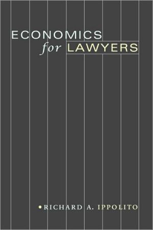
Economics for Lawyers

Economics for Lawyers\ \ By Richard A. Ippolito \ Princeton University Press\ Copyright © 2005 Princeton University Press\ All right reserved.\ ISBN: 978-0-691-12177-2 \ \ \ Chapter One\ Finding the Optimal Use of a Limited Income \ Main Economic Concepts\ 1. More is better.\ 2. Free choice is a valuable commodity.\ 3. Freedom to trade can make everyone better off.\ New Terms\ 1. Indifference curve\ 2. Diminishing marginal utility\ 3. Budget constraint\ 4. Optimal use of a limited income\ 5. Pareto efficiency\ 6. Pareto optimal allocation\ 7. Pareto efficient allocation\ 8. Edgeworth box diagram\ 9. Contract curve\ 10. Compensation principle\ 11. Substitution effect\ 12. Price effect\ 13. Income effect\ 14. Corner solution\ The best place to start the study of economics is with a model of consumer decisions. Each of us has a limited income and must make choices about how best to allocate it among competing uses. Compared to a bundle of goods and services that are given to us with a market value of $20,000, most of us would prefer to have a $20,000 income to spend as we want. Why? Because each of us has different preferences for different goods and services, and thus, the "value" of a dollar is higher if we have the opportunity to spend it as we please. The value of free choice is a central tenet in economics and provides the basisto understanding the concept of a demand curve.\ I. Indifference Curves\ I am going to pursue this problem in a simplified way. There are two goods, clothing and housing. There are no other uses of income, no savings and no taxes.\ A. THE MAIN QUESTION\ A person has $100 to spend during some period. Using the assumptions below, how much does he spend on clothing and housing?\ To answer this question, I need to introduce the concept of an indifference curve. An indifference curve merely tells us the various combinations of goods that make a particular consumer indifferent. Consider figure 1-1, panel (a). I assume that we can create a homogeneous unit of clothing, like yards of quality-adjusted material. This measure is shown on the horizontal axis. I also assume that we can create a homogeneous unit of housing, like number of quality-adjusted square feet, which I show along the vertical axis. Suppose we consider some combination of clothing and housing labeled B, which corresponds to 25 units of clothing and 50 units of housing. What other combinations of clothing and housing would make this consumer indifferent to this particular allocation?\ B. INDIFFERENCE CURVES SLOPE DOWNWARD\ We know that any bundle that has both more housing and more clothing must be superior to B, and thus, any such bundle cannot be on the same indifference curve. This inference follows from the axiom "More is better." The combinations of housing and clothing labeled II in the figure denote superior bundles as compared to B. Likewise, our consumer cannot be indifferent between the bundle labeled B and any combination of both less housing and less clothing, denoted by area IV in the figure. This means that the indifference curve passing though point B must pass through areas I and III. In other words, the indifference curve must be downsloping from left to right. Panel (b) in figure 1-1 shows one such indifference curve that satisfies this criterion.\ This particular indifference curve is unique to some hypothetical person that we are considering. To be concrete, suppose that we are drawing an indifference curve for Jane Smith, who in fact possesses the bundle of goods labeled A. This bundle comprises 100 units of housing and 12.5 units of clothing. And suppose that we quiz her as follows: if we take away some units of housing, leaving her with only 50 instead of 100, how many additional units of clothing would she require in order to be indifferent to bundle A? We suppose that she answers, 12.5 units, which I show in the diagram. This corresponds to bundle B. Thus, we know that bundles A and B must lie on the indifference curve. Note that over the relevant range, Jane is willing to give up an average of 4 units of housing for each unit of clothing she obtains.\ Assuming that we continue asking her questions like this, we could draw a line through all the points of her indifference curve, which I label as [U.sub.1] in panel (b). That is, [U.sub.1] describes all the combinations of clothing and housing that make Jane indifferent to bundle A; we can think of all these combinations as yielding the same utility to her, which is why I use the letter U to denote the indifference curve.\ C. OTHER THINGS TO KNOW ABOUT INDIFFERENCE CURVES\ A few other features of indifference curves are important to know: they (a) are convex to the origin, (b) are infinite in number, (c) never cross each other, and (d) different consumers have different indifference curves.\ Indifference curves are convex from the origin. This phenomenon is due to the concept of diminishing marginal utility, meaning that consumers attach a higher value to the first units of consumption of clothing or housing, and less value to marginal units of clothing or housing once they have an abundance of them. Thus, if Jane has lots of housing and little clothing, as for example at point A in the figure, she is willing to trade 50 units of housing for 12.5 units of clothing to form bundle B. But once she attains this bundle, she attaches less value to obtaining still more clothing and is more reluctant to give up more units of housing.\ For example, starting at point B, suppose that we take 25 units of housing from Jane, say from 50 to 25 units in the figure. She requires 25 more units of clothing to make her indifferent to bundle B. Bundle ITLITL denotes the new allocation. Over the range B to ITLITL, she is willing to sacrifice only 1 unit of housing to receive 1 unit of clothing, on average. Compare this to the move from point A to point B, where she was willing to give up four times as much housing for each unit of additional clothing, on average. The difference is that at point B, she already has a fair amount of clothing and thus is not willing to give up as much housing to obtain even more clothing.\ There are an infinite number of indifference curves. Panel (b) in figure 1-1 depicts a single indifference curve for Jane. That is, I started with bundle A and then drew an indifference curve through all the other bundles like B and ITLITL that yield the same utility to her. But suppose that Jane started with an allocation of goods labeled D. We know that this bundle of goods cannot be on indifference curve [U.sub.1] because in comparison to bundle B, for example, bundle D has both more clothing and more housing. Since more is better, then it follows that D must be on a higher indifference curve than B. Following the same reasoning, bundle E must be on a lower indifference curve.\ If we pursued the same experiment with Jane starting from bundle D as we did when she had bundle A, we could draw a second indifference curve running through bundle D in the figure. If we do, then we have an indifference curve labeled [U.sub.2]. Similarly, we could draw an indifference curve passing through point E, labeled [U.sub.0]. I show these indifference curves in figure 1-2, panel (a). [U.sub.2] is a higher indifference curve than [U.sub.1], and therefore any combination of housing and clothing on this curve is preferred to [U.sub.1]. Similarly, [U.sub.0] is a lower indifference curve than [U.sub.1], and therefore any combination of clothing and housing on this curve is inferior to [U.sub.1]. In reality, there are an infinite number of indifference curves. To keep the figures simple, we normally portray only two or three in the relevant range to illustrate a problem.\ Indifference curves do not cross. Each indifference curve is uniformly higher than the one below. Why? If they were not depicted this way, they would violate the rule of consistency. Consider panel (b) in figure 1-2. In this figure, I have drawn indifference curve [U.sub.1] and show points labeled F and G. I also portray indifference curve [U.sub.2] passing through point G. In drawing it this way, I am saying that bundle G yields the same amount of utility as bundle F. I also am saying that bundle G is the same as bundle H. But how can this be true, since bundle H has more housing and clothing than bundle F? This conundrum violates the consistency rule. We avoid this problem as long as we ensure that indifference curves never cross.\ Note that we can use this same idea to remind ourselves that any bundle on a higher indifference curve is superior to any bundle on a lower indifference curve. Consider panel (a) in figure 1-2. How can we be sure that bundle ITLITL is inferior to bundle D? We know this because bundle ITLITL offers the same utility as bundle B because they are on the same indifference curve. But bundle B clearly is inferior to bundle D because there are fewer units of housing and clothing in bundle B compared to D. Since ITLITL is the same as B, it follows that ITLITL also must be inferior to D. This is another application of the principle that more is better.\ Different consumers have different indifference curves. The indifference curves drawn for Jane are specific to her tastes. Ken Jones would have a different set of indifference curves depending on his tastes for clothing and housing. The basic look of his indifference curves would be similar to Jane's (downsloping, convex, etc.), but his trade-off of clothing and housing very likely would be somewhat different.\ II. Gains from Trade Using the Edgeworth Box Diagram\ With this small amount of modeling, we already can illustrate an important principle of economics-namely, the gains that result from trade. I demonstrate this concept in the simplest possible way. I assume that there are only two people, Jane and Ken. I have [ITLITL.sub.max] units of clothing and [H.sub.max] units of housing. I want to demonstrate the proposition that if I allocate these units in any arbitrary way to Ken and Jane, they almost always will make each other better off by trading. To do this, I need to show Jane and Ken's indifference curves on the same picture. This is done through the use of an Edgeworth box diagram.\ As a first step, I write Jane's indifference curves in figure 1-3, panel (a). I label [ITLITL.sub.max] and [H.sub.max] on the vertical and horizontal axis to remind myself that this is the maximum amount of clothing and housing available in the problem. In panel (b), I write Ken's indifference curves, but I do it in an odd way: I rotate it 180 degrees, so that his origin is diagonal to Jane's. In this picture, Ken has more clothing and housing as he moves away from his origin, as depicted by the arrows. Note that I also show [ITLITL.sub.max] and [H.sub.max] as the limits in this chart, so that the horizontal and vertical lengths of the axes are the same as Jane's.\ A. CONSTRUCTION OF THE BOX\ To create the "box," simply slide Ken's indifference curve map until it is superimposed onto Jane's. Note that the charts exactly fit together because the lengths of the axes are the same on Jane's and Ken's figures. I show these charts superimposed in figure 1-4. I label Ken's indifference curves [K.sub.i] and Jane's [J.sub.i]. Larger subscripts denote higher levels of utility. (Note that it is OK that Ken's and Jane's indifference curves cross each other, as long as Jane's and Ken's own indifference curves do not cross.)\ I want to illustrate the initial amount of clothing and housing that Ken and Jane have to start with. I could portray this allocation anywhere in the box, because the axes have been drawn so that no matter where I plot a point, the total amount of clothing and housing must add to the maximum amounts. For illustration, I arbitrarily allocate these goods as described by point A as shown in panel (a) of figure 1-5. Jane has lots of housing and not much clothing, while Ken has lots of clothing and not much housing.\ To solve the problem, I reintroduce some indifference curves. Recall that there are an infinite number of indifference curves for both Ken and Jane, and so by definition, we know that each has one curve passing through point A; and so I draw these curves as illustrated in panel (b), figure 1-5. Notice that these curves, when superimposed, look like a cigar. Ken's indifference curve is [K.sub.1] and Jane's is [J.sub.1].\ B. PARETO SUPERIOR TRADES\ It is immediately apparent that a trade could make either Ken or Jane or both better off without making either worse off. This trade involves Jane giving some housing to Ken, and Ken giving some clothing to Jane, meaning that the allocation moves in a southeast direction in the figure-that is, toward the fat part of the "cigar."\ For example, suppose that Ken and Jane trade in a way that moves their allocation from A to B. In this case, Ken is no worse off than at A, because he is on the same indifference curve; but Jane is clearly better off because at B she is on a higher indifference curve compared to point A (compare [J.sub.4] to [J.sub.1]). When a trade makes at least one participant better off and no participant is worse off, then it is said to be Pareto superior. Similarly, they could trade so that Jane is no worse off but Ken is better off. Ken gets the best deal without reducing Jane's utility at point ITLITL. The move from A to ITLITL also is Pareto superior. Many moves starting from A are Pareto superior.\ It is not possible to know exactly who is going to get the better deal in a trade. It depends on Jane's and Ken's relative bargaining power. Most likely, however, both will gain, and we can characterize the range of outcomes in which both can be better off compared to point A.\ To do this, I add a few more indifference curves in the relevant range in panel (a) of figure 1-6. Consider a move from point A to point D. In comparison to point A, both Ken and Jane each are on a higher indifference curve, and thus both have benefited from the trade. Clearly, the move from A to D represents a Pareto superior move. But at point D, both can trade again to further increase their utility. In general, as long as a "smaller cigar" can fit inside a "larger cigar" then in an Edgeworth box diagram, both consumers can be made better off by further trading. When does this process stop?\ C. THE CONTRACT CURVE: PARETO OPTIMAL ALLOCATIONS\ Once they reach a point where their indifference curves no longer form a "cigar" but are just tangent, then it is not possible for one to gain by further trade without making the other person worse off. One such outcome is depicted by point E. In general, this condition defines a Pareto optimal allocation. A Pareto optimal allocation exists when any possible move reduces the welfare of at least one person. Sometimes, a Pareto optimal solution is referred to as a Pareto efficient allocation. Likewise, a Pareto superior move sometimes is referred to as a Pareto efficient trade.\ So far, I have portrayed a solution for one arbitrary initial allocation of clothing and housing, namely A. For this allocation, I have shown at least three possible trading outcomes, namely B, ITLITL, and E in panel (a), figure 1-6, whereby at least one consumer is better off and none is worse off. Depending on how Jane and Ken bargain, we could have a solution anywhere along the segment CB in the figure. Any point along this segment has the characteristic that Jane's and Ken's indifference curves are tangent.\ What if the allocation we started with was not A but some other point in the Edgeworth box, for example, point G in panel (a)? Repeating the exercise for this allocation would lead us to some solution along the segment IH, which also is a segment along the contract curve.\ (Continues...)\ \ \ \ \ Excerpted from Economics for Lawyers by Richard A. Ippolito Copyright © 2005 by Princeton University Press. Excerpted by permission.\ All rights reserved. No part of this excerpt may be reproduced or reprinted without permission in writing from the publisher.\ Excerpts are provided by Dial-A-Book Inc. solely for the personal use of visitors to this web site. \ \

Ch. 1Finding the optimal use of a limited income1Ch. 2Demand curves and consumer surplus41Ch. 3Supply curves and the flow of resources : also sunk cost, opportunity cost, and transactions cost82Ch. 4Using demand and supply curves to evaluate policy127Ch. 5The economics of monopoly153Ch. 6Public goods and common resources : toward understanding the economics of property rights194Ch. 7Externalities : the Coase theorem228Ch. 8Pollution in the workplace : contract or externality? : an introduction to the rules of law247Ch. 9Lemons markets and adverse selection : signals, bonds, reputation, and tie-ins as solutions282Ch. 10Sorting as a solution to asymmetric information : coaxing market participants to divulge valuable information321Ch. 11Moral hazard and agency problems : when mispricing affects behavior348Ch. 12Game theory and related issues : strategic thinking when players are few and information is poor380

\ The Federal LawyerEconomics for Lawyers provides systematic instruction in economic theory relevant to law, starting with indifference curves and working its way through the basics of game theory. . . . [It] is a very good textbook. It is comprehensive, well-organized, clearly written, and very usable. . . . [T]he focus of the book is unique; I know of no other book that attempts to do the same thing.\ — G. Thomas Woodward\ \ \ \ \ The Federal Lawyer\ - G. Thomas Woodward\ Economics for Lawyers provides systematic instruction in economic theory relevant to law, starting with indifference curves and working its way through the basics of game theory. . . . [It] is a very good textbook. It is comprehensive, well-organized, clearly written, and very usable. . . . [T]he focus of the book is unique; I know of no other book that attempts to do the same thing.\ \ \ The Federal LawyerEconomics for Lawyers provides systematic instruction in economic theory relevant to law, starting with indifference curves and working its way through the basics of game theory. . . . [It] is a very good textbook. It is comprehensive, well-organized, clearly written, and very usable. . . . [T]he focus of the book is unique; I know of no other book that attempts to do the same thing.\ — G. Thomas Woodward\ \